Getting and Running the Application
Windows Software (Win 8.1 or higher)
IOLab-1.80.1605-setup.exe (recommended)IOLab_win32_1.80.1605.zip (old-style distribution for experts)
Download setup file and double click on it. If Windows issues a warning then tell it to Run Anyway. The application will be installed in your local AppData folder and a shortcut will be placed on your desktop. This video shows how the new installer works. Installation of a Driver may be required on some Windows 8 computers if the dongle is not detected.
IOLab_win32_1.79.1602.zip (old-style)
IOLab-1.78.1597-setup.exe
IOLab_win32_1.78.1597.zip (old-style)
IOLab-1.78.1590-setup.exe
IOLab_win32_1.78.1590.zip (old-style)
IOLab-1.76.1574-setup.exe
IOLab_win32_1.76.1574.zip (old-style)
IOLab-1.76.1573-setup.exe
IOLab_win32_1.76.1573.zip (old-style)
IOLab_win32_1.74.1560.zip
IOLab_win32_1.73.1556.zip
IOLab_win32_1.72.1546.zip
IOLab_win32_1.71.1545.zip
IOLab_win32_1.70.1530.zip
IOLab_win32_1.69.1505.zip
IOLab_win32_1.68.1498.zip
IOLab_win32_1.66.1493.zip
IOLab_win32_1.65.1491.zip
IOLab_win32_1.65.1484.zip
IOLab_win32_1.65.1472.zip
IOLab_win32_1.64.1457.zip
IOLab_win32_1.64.1452.zip
IOLab_win32_1.64.1450.zip
IOLab_win32_1.63.1447.zip
IOLab_win32_1.62.1445.zip
IOLab_win32_1.62.1443.zip
IOLab_win32_1.60.1429.zip
IOLab_win32_1.60.1426.zip
IOLab_win32_1.59.1418.zip
IOLab_win32_1.57.1399.zip
IOLab_win32_1.57.1388.zip
IOLab_win32_1.56.1379.zip
IOLab_win32_1.54.1371.zip
IOLab_win32_1.54.1365.zip
IOLab_win32_1.53.1359.zip
IOLab_win32_1.53.1338.zip
IOLab_win32_1.53.1327.zip
IOLab_win32_1.51.1310.zip
IOLab_win32_1.50.1298.zip
iOLabCEF_win32_0.38.1074.zip
Mac Software (For OSX 10.12 or higher)
IOLab_macosx_1.80.1615.zipExtract the application from the ZIP file and double-click on it. The first time you do this you may have to Ctrl-click on the application and choose Open to get past security. This video will show you how to download and run the Mac application.
IOLab_macosx_1.78.1597.zip
IOLab_macosx_1.78.1590.zip
IOLab_macosx_1.76.1573.2.zip
IOLab_macosx_1.74.1560.zip
IOLab_macosx_1.73.1556.zip
IOLab_macosx_1.72.1546.zip
IOLab_macosx_1.71.1545.zip
IOLab_macosx_1.70.1530.zip
IOLab_macosx_1.68.1498.zip
IOLab_macosx_1.66.1493.zip
IOLab_macosx_1.65.1491.zip
IOLab_macosx_1.65.1484.zip
IOLab_macosx_1.65.1472.zip
IOLab_macosx_1.64.1457.zip
IOLab_macosx_1.64.1452.zip
IOLab_macosx_1.64.1450.zip
IOLab_macosx_1.63.1447.zip
IOLab_macosx_1.62.1445.zip
IOLab_macosx_1.62.1443.zip
IOLab_macosx_1.60.1429.zip
IOLab_macosx_1.60.1426.zip
IOLab_macosx_1.59.1418.zip
IOLab_macosx_1.57.1399.zip
IOLab_macosx_1.57.1388.zip
IOLab_macosx_1.56.1379.zip
IOLab_macosx_1.54.1371.zip
IOLab_macosx_1.54.1365.zip
IOLab_macosx_1.53.1359.zip
IOLab_macosx_1.53.1338.zip
IOLab_macosx_1.53.1327.zip
IOLab_macosx_1.51.1310.zip
IOLab_macosx_1.50.1298.zip
iOLabCEF_macosx_0.38.1074.zip
Python Development
Python 2.7 IOLab API, Python 3 IOLab APIThese are links to Python libraries that enables primitive stand-alone communication with iOLab. They are NOT designed to replace the highly capable application you can download for Windows and Mac at the above links, but rather to enable interested people to play with the guts of the iOLab system at a programming level. If you want to get involved with further development of this fun python resource please send me an email at mats.selen@gmail.com.
Selected Release Notes
-
1.80.1615 for Mac (June/17/2024):
Fixed issue where code hung on a blank screen on some machines running OSX Sonoma. -
1.80.1605 (Feb/21/2021):
Fixed rare Windows dongle detection issue caused by WMI errors on some Win-10 computers.
See ChangeLog for details. -
1.79.1602 (Sept/27/2020):
Mac version should work for all OSX.
Windows version has bug fix. -
1.78.1597 (Aug/16/2020):
Several improvemments and a bug-fix. -
1.78.1590 (Aug/6/2020) (Replaced 1.77.1584):
Added RF Signal Strength chart (RSSI).
Added local Bz variable to config.json for improved magnetometer calibration. -
1.76.1574 (Feb/9/2020):
Rebuilt dongle-detection code for compatibility with 32 bit machines. -
1.76.1573 (Jan/16/2020):
Implemented windows installer with code signing certificate. Several other improvements. -
1.74.1560 (Sep/17/2019):
Added new sensor to sample A1/A2/A3 at 800 Hz. Added lesson player support for outputs pins on header. -
1.70.1530 (Feb/6/2019):
Shuts remote off after 5 minutes of inactivity (adjustable). Bug-fix for PDF export on Mac. -
1.66.1493 (Sept/13/2018):
No driver installation required if using (Windows 8 or 10).
Quick Start Guide
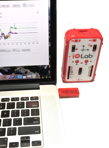
- Plug in the dongle and turn on the iOLab device.
- Start the application as described above (slightly different for Mac & PC).
- Select the sensors you want to read out from the list on the left - the system readout will be optimized for the selected sensors and charts to display the data from the selected sensors will created.
- Click on the Record button to start data acquisition, and click on the Stop button to stop.
- The Data Smoothing button selects how many points are included in the smoothing average.
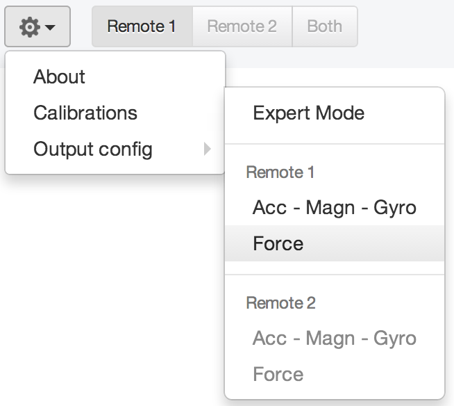
Calibrating Your Sensors
It is important to calibrate your devices force probe and accelerometer. Click the reset button ![]() twice, then select the sensor to calibrate from the tools menu:
twice, then select the sensor to calibrate from the tools menu:
Restoring & Saving Your Data
Each time data is acquired it is automatically saved to the Documents/iOLab-WorkFiles/rawdata folder on your local computer. You can restore any previous acquisition by clicking on the file icon and selecting the data you want.
You can export the data from any chart to a CSV (Excel) file by clicking on the export icon. The data is saved to the Documents/iOLab-WorkFiles/export folder on your local computer.
Navigating Your Plots
When the "graph" icon is selected (the default), the mouse is used to select regions for analysis. Left-click and dragging will select a region the region (shaded blue) for which averages are displayed. Left-clicking without dragging will move the FFT region (shaded gray) when FFT analysis is enabled.
When the "magnifying glass" icon is selected, the mouse is used to select a rectangular region for zooming. Double clicking on the plot in this mode will reset the zoom to the initial default values. Zooming in on one of the plots sets the time axis for all of the plots to be set to the same region as the plot being zoomed on, keeping the time axis the same on all plots.
When the "compass" icon is selected the mouse is used to pan left & right & up & down on a plot. Moving one plot horizontally causes all of the plots to be moved horizontally, keeping the time axis the same on all plots.